How to represent a 3D Gaussian Function with ROS rviz

The probabilistic functions are very usual in robotics to represent the certainty of states and observations. The most typical and used probabilistic function is the Gaussian function. Everybody who knows what is this immediately imagine a pretty bell which describes the samples nature.

In the one-dimensional case, a simple tuple mean, variance is enough information to imagine how the samples are behaving. This tuple can be also reinterpreted as an interval where the samples most probably are located. For higher dimensions the \mu it is clear, but the equivalent element to describe the diversity, the covariance matrix  it is much lesser intuitive for most of people. The trick is imagine the ND gaussian bell as NDimensional ellipse. The shape and rotation of this ellipse is described by the covariance matrix. In this way the diversity of the distribution is intuitive.

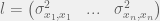
It is extremely interesting to see and understand the relationship with the rotation and scale of the ellipsoid. If we define as the rotation transform of the ellipsoid and is a vector with the variances in the local frame of the ellipse (much easier to imagine)  , then the relationship between and is this:

This have important implications because if you want to synthesizer a gaussian belief from a theoretical model can be hard imagine the covariance matrix values but it is very easy to think in an ellipse with a rotation and scale.

The inverse operation is also useful. For instance if you have a covariance matrix obtained experimentally and you wish to make a geometric interpretation of the distribution or just plot it, you can obtain the rotation matrix and the scale vector . Then the it is needed to compute the eigenvectors and eigenvalues. That is because:

and

Of course notice that if number of eigenVectors is lower than the dimensionality of the problem is because the ellipse is infinitely slim and as a consequence the determinant and then the matrix is singular. This means that one dimension should be removed if you want to compute likelihoods over that gaussian function.

Here I show how to represent a 3D gaussian function with ROS and rivz:

And here the code in python. Discussion about this subject in: http://answers.ros.org/question/2043/plot-a-gaussian-3d-representation-with-markers-in:

import roslib
roslib.load_manifest ("gaussian_markers")
import rospy
import PyKDL
from visualization_msgs.msg import Marker, MarkerArray
import visualization_msgs
from geometry_msgs.msg import Point
import numpy
from numpy import concatenate

#syntetic 3-D Gaussian probabilistic model for sampling
covMatModel =[[10, 10, 0],[10, 1, 0],[0, 0, 4]]
meanModel =[10, 10, 10]

#used to paint the autovectors
def markerVector(id,vector,position):
	marker = Marker ()
	marker.header.frame_id = "/root";
	marker.header.stamp = rospy.Time.now ()
	marker.ns = "my_namespace2";
	marker.id = id;
	marker.type = visualization_msgs.msg.Marker.ARROW
	marker.action = visualization_msgs.msg.Marker.ADD
	marker.scale.x=0.1
	marker.scale.y=0.3
	marker.scale.z=0.1
	marker.color.a= 1.0
	marker.color.r = 0.33*float(id)
	marker.color.g = 0.33*float(id)
	marker.color.b = 0.33*float(id)
	(start,end)=(Point(),Point())

	start.x = position[0]
	start.y = position[1]
	start.z = position[2]
	end.x=start.x+vector[0]
	end.y=start.y+vector[1]
	end.z=start.z+vector[2]

	marker.points.append(start)
	marker.points.append(end)
	print str(marker)
	return marker

rospy.init_node ('markersample', anonymous = True)
points_pub = rospy.Publisher ("visualization_markers", visualization_msgs.msg.Marker)
gauss_pub = rospy.Publisher ("gaussian", visualization_msgs.msg.Marker)

while not rospy.is_shutdown ():
	syntetic_samples = None

	#painting all the syntetic points
	for i in xrange (10, 5000):
		p = numpy.random.multivariate_normal (meanModel, covMatModel)
		if syntetic_samples == None:
			syntetic_samples =[p]
		else:
			syntetic_samples = concatenate ((syntetic_samples,[p]), axis = 0)

		marker = Marker ()
		marker.header.frame_id = "/root";
		marker.header.stamp = rospy.Time.now ()
		marker.ns = "my_namespace2";
		marker.id = i;
		marker.type = visualization_msgs.msg.Marker.SPHERE
		marker.action = visualization_msgs.msg.Marker.ADD
		marker.pose.position.x = p[0]
		marker.pose.position.y = p[1]
		marker.pose.position.z = p[2]
		marker.pose.orientation.x = 1
		marker.pose.orientation.y = 1
		marker.pose.orientation.z = 1
		marker.pose.orientation.w = 1
		marker.scale.x = 0.05
		marker.scale.y = 0.05
		marker.scale.z = 0.05
		marker.color.a = 1.0
		marker.color.r = 0.0
		marker.color.g = 0.0
		marker.color.b = 0.0
		points_pub.publish (marker)

	#calculating Gaussian parameters
	syntetic_samples = numpy.array (syntetic_samples)
	covMat = numpy.cov (numpy.transpose (syntetic_samples))
	mean = numpy.mean ([syntetic_samples[: , 0], syntetic_samples[: , 1], syntetic_samples[:, 2]], axis = 1)

	#painting the gaussian ellipsoid marker
	marker = Marker ()
	marker.header.frame_id ="/root";
	marker.header.stamp = rospy.Time.now ()
	marker.ns = "my_namespace";
	marker.id = 0;
	marker.type = visualization_msgs.msg.Marker.SPHERE
	marker.action = visualization_msgs.msg.Marker.ADD
	marker.pose.position.x = mean[0]
	marker.pose.position.y = mean[1]
	marker.pose.position.z = mean[2]

	#getting the distribution eigen vectors and values
	(eigValues,eigVectors) = numpy.linalg.eig (covMat)

	#painting the eigen vectors
	id=1
	for v in eigVectors:
		m=markerVector(id, v*eigValues[id-1], mean)
		id=id+1
		points_pub.publish(m)

	#building the rotation matrix
	eigx_n=PyKDL.Vector(eigVectors[0,0],eigVectors[0,1],eigVectors[0,2])
	eigy_n=-PyKDL.Vector(eigVectors[1,0],eigVectors[1,1],eigVectors[1,2])
	eigz_n=PyKDL.Vector(eigVectors[2,0],eigVectors[2,1],eigVectors[2,2])
	eigx_n.Normalize()
	eigy_n.Normalize()
	eigz_n.Normalize()
  	rot = PyKDL.Rotation (eigx_n,eigy_n,eigz_n)
	quat = rot.GetQuaternion ()

	#painting the Gaussian Ellipsoid Marker
	marker.pose.orientation.x =quat[0]
	marker.pose.orientation.y = quat[1]
	marker.pose.orientation.z = quat[2]
	marker.pose.orientation.w = quat[3]
	marker.scale.x = eigValues[0]*2
	marker.scale.y = eigValues[1]*2
	marker.scale.z =eigValues[2]*2

	marker.color.a = 0.5
	marker.color.r = 0.0
	marker.color.g = 1.0
	marker.color.b = 0.0

	gauss_pub.publish (marker)
	rospy.sleep (.5)